|
|
DevelopmentSega Master System / Mark III / Game Gear |
Home - Forums - Games - Scans - Maps - Cheats - Credits |
YM 2413 Reverse Engineering Notes 2016 - 07 - 16
by andete. Original documents available at: https://github.com/andete/ym2413/tree/master/results
<< YM2413 Reverse Engineering Notes 2016-02-10 | YM2413 Reverse Engineering Notes | YM2413 Reverse Engineering Notes 2017-01-26 >>
Introduction
It's (again) been over half a year since my last post. I'm almost ashamed about how slowly this is progressing. But then better slow progress than abandoning the project.
In previous posts we've already fairly well investigated isolated YM2413 components. Now it's time to start putting them together. Though instead of immediately building a model that includes everything we've learned, we'll build the model in smaller steps.
This initial partial model will include:
- Modulator and carrier operators connected together.
- Feedback stuff in the modulator.
- Channel volume
- Key Scale Level
There is partial support for:
- Envelope level, the current level is taken into account, but the level does not change over time.
- Similar for LFO AM: the level is taken into account, but it remains fixed in time.
The most important missing pieces (that we did already investigate) are:
- Evolving envelope level.
- Evolving LFO AM level.
- Selectable waveform (though I'll add it at the end of this post).
- Channel frequency and LFO PM.
Initial partial model
The following c++ code is pieced together from code snippets from previous posts. If you (re)read those posts, there shouldn't be any surprises in this code.
Remember that this code is more geared towards clarity or to how the hardware (likely) implements the algorithm rather than towards an efficient software implementation.
uint16_t logsinTable[256];
void initTables() {
for (int i = 0; i < 256; ++i) {
logsinTable[i] = round(-log2(sin((double(i) + 0.5) * M_PI / 256.0 / 2.0)) * 256.0);
expTable[i] = round((exp2(double(i) / 256.0) - 1.0) * 1024.0);
}
}
uint16_t lookupSin(uint16_t val) {
bool sign = val & 512;
bool mirror = val & 256;
val &= 255;
uint16_t result = logsinTable[mirror ? val ^ 0xFF : val];
if (sign) result |= 0x8000;
return result;
}
int16_t lookupExp(uint16_t val) {
bool sign = val & 0x8000;
int t = (expTable[(val & 0xFF) ^ 0xFF] << 1) | 0x0800;
int result = t >> ((val & 0x7F00) >> 8);
if (sign) result = ~result;
return result;
}
int main()
{
initTables();
int tl = 63; // 0..63
int fb = 0; // 0..7
int vol = 0; // 0..15
int kslM = 0; // 0 .. 112
int kslC = 0; // 0 .. 112
int envM = 127; // 0 .. 127
int envC = 128; // 0 .. 127
int amM = 0; // 0 .. 13
int amC = 0; // 0 .. 13
int16_t p0 = 0;
int16_t p1 = 0;
for (int i = 0; i < 1024; ++i) {
auto f = fb ? (p0 + p1) >> (8 - fb) : 0;
auto sM = lookupSin((i - 1) + f);
auto attM = 2 * tl + kslM + envM + amM;
auto m = lookupExp(sM + 16 * attM) >> 1;
p1 = p0; p0 = m;
auto sC = lookupSin(i + 2 * m);
auto attC = 8 * vol + kslC + envC + amC;
auto c = lookupExp(sC + 16 * attC) >> 4;
cout << 255 - c << endl;
}
}
Observation + 1st experiment
While creating this model I noticed that in this implementation the output of a channel never stops changing (even when assuming that the envelope level does go to a maximum over time). At the very least (when the envelope reaches a very high attenuation level) the signal keeps toggling between plus and minus zero.
Let's measure how the real hardware behaves. I ran the following experiment:
| Operator | AM | PM | EG | KR | ML | KL | TL | WF | FB | AR | DR | SL | RR |
|---|---|---|---|---|---|---|---|---|---|---|---|---|---|
| modulator | 0 | 0 | 0 | 0 | 00 | 0 | 63 | 0 | 0 | 15 | 15 | 15 | 15 |
| carrier | 1 | 0 | 0 | 0 | 02 | 0 | 0 | 08 | 02 | 00 | 02 |
block=0, fnum=256, volume=0
With these settings each sine period takes 1024 samples and every 4096 samples the envelope level increases by one. 1024 samples per sine was chosen because the sine-table has 1024 entries (see previous posts), thus we can see all details of the 'sine shape'. The slow envelope setting was chosen so that each level contains 4 repeated sines and we don't have to worry about transition effects (e.g. we can look at the 'middle two' sine waves).
Here are the results. The first image shows the full signal. The second image zooms in on the tail of the signal (the rectangle marked in green in the 1st image).


So eventually the real YM2413 signal stops changing. In the c++ model above this is not the case. Let's try to figure out when exactly it stops.
From previous results we know that for envelope level 111 the signal varies between +/-2 (6 values, +2, +1, +0, -0, -1, -2). All later envelope levels only vary between +/-1 (4 values, +1, +0, -0, -1). So by only measuring the peak amplitude we cannot distinguish levels 112-127.
However, in this experiment, every 4096 samples the envelope level increases by one, and it's relatively easily to locate level 111 (6 instead of 4 distinct output values). From this we can calculate that the signal stops changing at the point where we expect envelope level 124.
So in a way we 'counted' the expected envelope level (count from 112 to 124 every 4096 samples). There's an alternative way to obtain the same result (which will also be useful later on in this post): we can look at the 'shape' of the 'sine' wave.
The following image zooms in even more on the above signal. In green and red I've indicated to peak-widths of the signal at places where we respectively expect envelope level 112 (the first level with only 4 distinct output values) and envelope level 113 (4096 samples after the green peak).
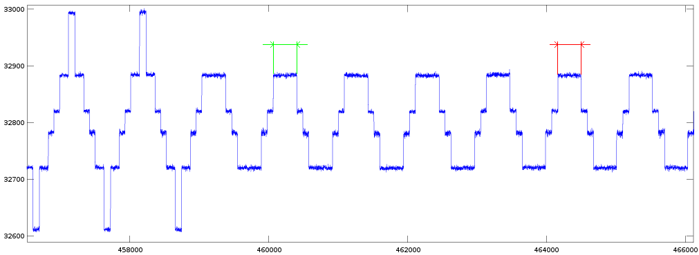
The widths of those peaks are respectively 342 and 332 samples (as expected a higher attenuation level results in a more narrow peak). The waveforms generated by the c++ model for the corresponding envelope levels have the same peak-widths.
The following table gives the peak-width for more envelope levels (for all the levels where the output only varies between +/-1). For all these levels the measured width matches exactly with the predicted width by the model.
    level || model | measured-peak-width
   -------++-------+---------------------
     112  ||  342  |  342
     113  ||  332  |  332
     114  ||  324  |  324
     115  ||  314  |  314
     116  ||  304  |  304
     117  ||  294  |  294
     118  ||  282  |  282
     119  ||  270  |  270
     120  ||  256  |  256
     121  ||  240  |  240
     122  ||  224  |  224
     123  ||  206  |  206
     124  ||  186  |  186 (*)
     125  ||  162  |  162 (*)
     126  ||  132  |  132 (*)
     127  ||   94  |   94 (*)

  (*) So far we don't have any measurements yet for levels 124-127, they will
      come later.
So this table allows to derive the envelope level for low-amplitude signals without having to know how the envelope evolves (increases by 1 every 4096 samples in this example) or without to need for a known reference point (level 111 is easy to locate in this example).
2nd experiment, lower volume
In the above experiment the signal stops changing once the carrier envelope reaches level 124. At that point the signal remains constant at value +0 (not -0, nor alternating between +/-0, nor does it keep the sign of the last output value). But what if we attenuate the signal more, does the signal then sooner take on a constant value?
The signal can be attenuated by:
- Lowering the volume.
- Using LFO amplitude modulation.
- Using the Key Scale Level (KSL) feature.
I tested all 3, all give the same result, so I'll only (or mostly) discuss the first alternative (lowering the volume) in more detail.
The next experiment is the same as the previous one, except that the channel volume is now set to 8 (was 0, higher value means lower volume, 3dB per step). The result is visible in the following graph.

Overall the shape of this graph is similar to the one from the previous experiment, but the volume is quite a bit lower (check the range on the y-axis).
Before discussing this result in more detail, let's first clarify some
terminology. While discussing the previous result I always talked about the
envelope level (of the carrier). This corresponds with the 'envC' variable in
the c++ model. But what we actually measure is the total attenuation level (the
'attC' variable in the model). Though we have:
attC = 8 * vol + kslC + envC + amC;
and in the previous experiment
vol=0, kslC=0, amC=0
so there was no difference between the envelope and the total attenuation
level. But now we have vol=8, so I'll be more careful in distinguishing both.
The first thing we see in this second experiment is that there is a very long tail where the signal only varies between +/-1. By measuring the total length of the signal (the part where it keeps changing) and dividing that by 4096 (the number of samples per envelope step), we obtain the value '124'. So again it seems that the output remains constant at +0 once the carrier envelope reaches level 124.
If we zoom in on this tail (not shown), and compare the widths of the peaks with the values from the above table, we can derive the total attenuation level. This level starts at 112 and increases by one every 4096 samples until it reaches level 127 (so here we can measure the peek-widths for levels 124-127, and they indeed match the predictions). Beyond this point the total attenuation level remains at 127 (until the envelope level reaches 124).
So far all experiments used a monotonically increasing total attenuation level. I also did an experiment with LFO AM (not shown). That results in a periodically increasing/decreasing attenuation level. Combined with a low volume it's possible to create a situation where the total attenuation level would periodically go below and above level 127. Though when actually measuring this, we again see that the total attenuation level never goes above 127.
An intermediate conclusion:
- It seems the total attenuation level is clipped at 127.
- For envelope levels 124 or above (easily tested in hardware by (only) checking the top 5 bits) the output is constant +0.
Extending the model (the carrier part) with this new information gives:
if ((envC & 0x7C) != 0x7C) {
auto sC = lookupSin(i + 2 * m);
auto attC = min(127, 8 * vol + kslC + envC + amC);
c = lookupExp(sC + 16 * attC) >> 4;
}
3rd experiment, modulator
The experiments so far only looked at the carrier part. But what about the modulator? We know that the same hardware is used (time multiplexed) for both the carrier and the modulator operator calculations. So it's very likely the clipping of the total attenuation level (at 127) is also done for the modulator (because it's an 'internal' part of the operator calculation).
However making the output constant +0 is most easily implemented in hardware as a selection at the end:
- The hardware always calculates the intermediate result.
- At the end there's a mux that, depending on the envelope level, selects between this intermediate result or the constant value +0.
Because this selection is done at the end, it could either be part of the (shared) operator calculation, or it could be on a hardware path that's specific for the carrier. Let's try to figure out which of these two alternatives was chosen by the YM2413 engineers.
I designed an experiment with these parameters:
| Operator | AM | PM | EG | KR | ML | KL | TL | WF | FB | AR | DR | SL | RR |
|---|---|---|---|---|---|---|---|---|---|---|---|---|---|
| modulator | 0 | 0 | 0 | 0 | 02 | 0 | 00 | 0 | 0 | 08 | 02 | 00 | 02 |
| carrier | 0 | 0 | 1 | 0 | 02 | 0 | 0 | 15 | 15 | 15 | 00 |
The changes compared to the previous experiments are:
- After a (short) initial transition, the carrier envelope remains at a constant level 120. (In the previous experiment it gradually changed from 0 to 123).
- The modulator envelope now changes from 0 to max, with 4096 samples per step.
- In the previous experiment we wanted to suppress modulation, now we want it to be visible. So we set TL=0 (instead of TL=63). (Actually, with hindsight, the value of TL doesn't really matter).
I'm not showing a graph of the full output because it doesn't teach us much: Roughly over the full graph, 570k samples, the signal varies between +/-1. More to the start (low modulator envelope attenuation levels) the signal varies more rapidly, more to the end (high modulator envelope attenuation levels) the signal is *almost* a sine wave (though of course a sine approximated with only integer values between +1 and -1).
Instead I'll show a small part of this signal zoomed near the end:

There are two transitions visible from +0 to -0, respectively encircled in green and in red. The following two graphs zoom-in on these two regions.


In the green region there's a hiccup: the signal goes +0, -0, +0, -0. While in
the red region the +0 to -0 transition is clean.
What does this mean? To figure this out, let's go back to the c++ model. What does it predict for carrier envelope level 120 and modulator envelope level 127. The prediction is shown in this graph:

Even for very high modulation attenuation levels (meaning little modulation) we still get a single 'hiccup' in the +0 to -0 transition. These hiccups are identical for modulation levels 123..127. If we instead keep the output of the modulator constant at +0 the predicted transition is clean.
This means that in the green region there still is some modulation, but in the red region there's not. From the shape of the (green) signal we cannot determine the modulator envelope level, but the red region is located near sample 124x4096. So that's a strong indication that also the modulator output is kept at a constant value +0 once the modulator envelope level reaches value 124.
A bit of speculation
Why does the output already stop changing when level 124 is reached instead of going up to 127? One (minor?) reason could be that only testing 5 bits is a little cheaper in hardware compared to testing all 7 bits (though at the cost of some dynamic range).
Another (more important?) reason might be that for very fast envelope rates the envelope increases by 2 (instead of just 1) every sample. Thus the envelope level can go 124 -> 126 -> 128 (or 125 -> 127 -> 129). But because the value is stored in only 7 bits, it actually goes 124 -> 126 -> 0. So value 127 is never reached and the 7-bit-stop-condition never triggers. This could be solved by adding clipping logic to the level-increment, but a cheaper solution is to simply not test the lowest bit. Though this doesn't explain why the hardware only tests 5 bits (instead of 6).
Even more speculative: YM2413's big brother is the YM3812 (OPL2). In that chip the envelope level can also increase in steps of 4 per sample (there the envelope also has a higher resolution). In that case the above trick only works if 2 bits are ignored. Perhaps this detail was kept when deriving the YM2413 from the YM3812 design?
Waveform details
The YM2413 has two different basic shapes for the waveform:
- A (full) sine-wave.
- Half a sine-wave; the negative part is replaced with zeros.
I've already investigated this half-sine in previous posts. I had measured that indeed the positive part of the sine is kept and the negative part is replaced with zeros. But now I realize I've never checked whether those zeros are +0 or -0.
With only small changes to the previous experiments, I could measure this:

This only shows 3 distinct output values (ignoring measurement noise). These values are +1, +0 and -0 (remember that in my test-setup lower ADC values correspond to positive YM2413 values). When I measure the lengths of the segments with value -0, they are exactly 512 samples long (exactly half a period in this experiment).
This means that for the half-sine waveform, the absolute value of the 2nd part is set to zero, but the sign still toggles.
Updated model
With the refinements discovered in this post, we can now update the (partial) c++ model. It looks like this:
uint16_t logsinTable[256];
void initTables()
{
for (int i = 0; i < 256; ++i) {
logsinTable[i] = round(-log2(sin((double(i) + 0.5) * M_PI / 256.0 / 2.0)) * 256.0);
expTable[i] = round((exp2(double(i) / 256.0) - 1.0) * 1024.0);
}
}
// input: 'val' 0..1023 (10 bit)
// output: 1+12 bits (sign-magnitude representation)
uint16_t lookupSin(uint16_t val, bool wf)
{
bool sign = val & 512;
bool mirror = val & 256;
val &= 255;
uint16_t result = logsinTable[mirror ? val ^ 0xFF : val];
if (sign) {
if (wf) result = 0xFFF; // zero (absolute value)
result |= 0x8000; // negate
}
return result;
}
int16_t lookupExp(uint16_t val)
{
bool sign = val & 0x8000;
int t = (expTable[(val & 0xFF) ^ 0xFF] << 1) | 0x0800;
int result = t >> ((val & 0x7F00) >> 8);
if (sign) result = ~result;
return result;
}
int main()
{
initTables();
int tl = 0; // 0..63
int fb = 0; // 0..7
int vol = 0; // 0..15
int kslM = 0; // 0 .. 112
int kslC = 0; // 0 .. 112
int envM = 127; // 0 .. 127
int envC = 120; // 0 .. 127
int amM = 0; // 0 .. 13
int amC = 0; // 0 .. 13
bool wfM = 0;
bool wfC = 1;
int16_t p0 = 0;
int16_t p1 = 0;
for (int i = 0; i < 1024; ++i) {
// modulator
auto f = fb ? (p0 + p1) >> (8 - fb) : 0;
int m = 0; // corresponds to '+0'
if ((envM & 0x7C) != 0x7C) {
auto s = lookupSin((i - 1) + f, wfM);
auto att = min(127, 2 * tl + kslM + envM + amM);
m = lookupExp(s + 16 * att) >> 1;
}
p1 = p0; p0 = m;
// carrier
int c = 0; // corresponds to '+0'
if ((envC & 0x7C) != 0x7C) {
auto s = lookupSin(i + 2 * m, wfC);
auto att = min(127, 8 * vol + kslC + envC + amC);
c = lookupExp(s + 16 * att) >> 4;
}
cout << 255 - c << endl;
}
}
Next steps
In the next post(s) I'll probably complete this partial model with more and more features (features that have already been investigated in isolation). Though I don't know yet which feature(s) I'll add first. Possibly along the way I'll notice more corner cases that need further investigation.
Once the model is reasonably complete we can start comparing it against settings from the instrument ROM.
<< YM2413 Reverse Engineering Notes 2016-02-10 | YM2413 Reverse Engineering Notes | YM2413 Reverse Engineering Notes 2017-01-26 >>
